
Creating and Understanding
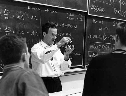
The following line was found scrawled on Richard Feynman’s blackboard after he died:
“What I cannot create, I do not understand.”
It would be a fitting gravestone epitaph, coming from someone who was so fanatical about understanding things.
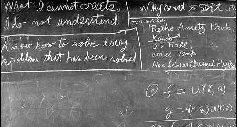
Feynman’s blackboard at Caltech
Unfortunately, the corollary, “What I can create, I do understand” is not always true. We only need to turn to modern developments in Artificial Intelligence to find an important example of this.
Neural Networks and Emergent Behaviour
For many years, neural networks have been taking over from rule-based systems in AI. One of the reasons most often cited for this development is that it is extremely labour-intensive to build a rule-based system.
I think this reason, although important, misses the true mark by quite a bit. The really exciting thing about neural nets is that they are capable of discovering patterns that humans have not themselves already discovered: effectively, new knowledge. A rule-based system, coded by hand, can only represent extant knowledge.
That’s great, but where is all this “new knowledge” coming from? And do we understand it?
Virtually all neural-net technologies currently employed in Artificial Intelligence rely heavily on emergent behaviour to do their heavy lifting. Emergent behaviour is that nifty bit of “something for nothing” that occurs when comparatively simple systems suddenly spit out surprisingly complex or information-rich results. Snowflakes and the feather-like patterns on your car windshield on a cold morning, which arise from just cold moist air, are one archetypal example. And, to a crude approximation, life from “some warm little pond”, as Darwin suggested in an 1871 letter to Joseph Hooker, is another.
In both cases, something much more complex emerges from the casual interactions of a substantial number of relatively basic sub-units. Simple water molecules combine to produce fantastic fractal patterns; a carbon/water/trace elements-laced soup produces simple chemical replicators, and we find ourselves on the long road to Life….
In the case of the neural networks, now ubiquitously employed in AI, the same type of emergent behaviour occurs. Let’s see how.
The Anatomy of a Simple Neural Network
These nets are typically built in layers of “software neurons” that are stacked one on top of the other. Schematically, input is shown as being entered in the bottom of the net, with some result emerging as output at the top. In all but the most trivial nets, there are several, sometimes many layers of neurons in between, called “hidden layers”, where the real work is done. So the whole thing is a stack, with processing moving in a wave from bottom to top.
Let’s take classifiers as an example.
The simplest of such nets are called “feed-forward”: the only wiring permitted is between a neuron and its neighbours in the layer immediately above it. So although there may be a one-to-many relation, wiring is always directed upwards. There is no horizontal wiring (between neurons of the same layer), and there is no recurrence (no looping back to the level below).
In the most basic cases, the hidden layers are all structurally the same (although they evaluate different abstractions of the original input). The structure of the input layer is dependent upon the structure of the input data itself. The output layer, at the very top, typically winnows down to the number of possible classification outputs.
Here is a schematic of an absurdly simplified image classification system, that categorizes an imagine into one of two different categories:
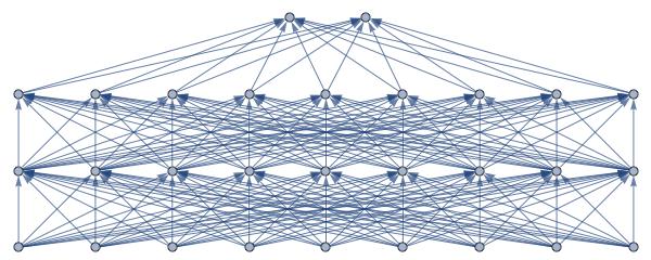
Neural net schematic
Pre-processing of the system (not shown in the schematic, and done to simplify input and speed up processing) takes an original image, and chops it up into some standardised pixel block of size. For example, a simple 24 by 24 pixel image could be subdivided into 8 by 8 chunks. Such a mapping can cover the whole image with 9 non-overlapping blocks. Hence the 9 neurons you find in the bottom, which form the input layer of the schematic. The system processes each image through 2 hidden layers, and classifies it to two possible options. So at the very top, we find just 2 neurons on our output layer.
Of course the relatively simple structure above hides a world of complexity. Some sophisticated processing happens at each neuron, as input moves up through the system in a layer-by-layer wave. Typically, each layer is responsible for processing some abstract aspect of the image, with each neuron in a layer responsible for evaluating a pixel block according to characteristics of its layer’s abstraction.
A Noddy Worked Example
Let’s work through a ridiculously simplified example.
Imagine the task of the system is to import images (photos or artwork) and estimate whether each depicts a day or a night scene. It outputs two probability values: real numbers for both day and night, the two adding to exactly 1.0. The “winner” is whichever has the highest probability score.
Imagine the first hidden layer contains neurons that examine an individual pixel block for shades of blue that might indicate a daytime sky; it is not perfect — there are plenty of shades of blue, and not all of them unambiguously imply sky — but it is a reasonable approximation. A system of numeric weights is assigned to different shades. Lots of the right shades of blue mean a high probability of the current image being a daytime shot; not much blue implies a lower probability.
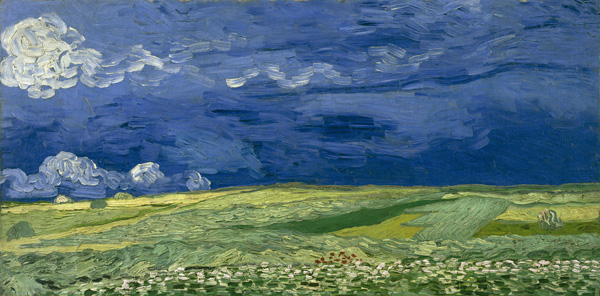
van Gogh – Wheatfield Under Thunderclouds (1890)
The next layer might look for colours associated with incandescent bulbs being lit. Lots: more likely night; little, more likely day. So each little neuron returns its “Vote: Day or Night” as a probability score (again, a pair of reals, adding to exactly 1.0).
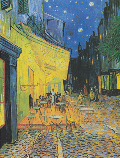
van Gogh – Terrasse on the Place du Forum (September 1888)
N.B. – In this, a “binary” classifier, where there are only two possible outputs, just one score would actually need to be passed forward, the other being inferred because the two must add up to 1.0. The moment there are more than two options — day, twilight, night, for example — a score for each output class must be maintained throughout the system. It is not hard to see that a real-world AI, tasked with something like evaluating patient symptoms, and diagnosing from many tens or even hundreds of different possible diseases, can rapidly become a very complex system indeed. But lets continue the story for our simple day/night model.
The probability scores from the first layer get passed up to the next layer, where they are combined with the calculations of each neuron there, using an equation to meld the two. So as processing proceeds up the layers of the net, the system is refining its “day/night” estimate, on a block-by-block, neuron-by-neuron basis. Eventually we arrive at the output layer, where all blocks are consolidated into the two output neurons, representing “day” and “night”. Some function averages all the scores in the last hidden layer, and effectively “votes” for day or night. Here we might find the voting has resulted in a score of Day: 0.891; Night: 0.109. Verdict: this is very likely a daytime shot.
We Can Build It; But Do We Understand It?
We certainly can build these things. Indeed, the vast majority of useful neural nets are orders of magnitude more complex than this, with many hidden layers, and thousands or even millions of neurons in total. We build them, and they work.
So, imagine we’ve built one. In what sense do we understand it?
Well, there is a level at which the explanation above proves our understanding is tolerably good. But in fact the explanation hides a lot of important detail.
First, any significant neural net is not pre-programmed at the layer-level to look for obvious characteristics like blue sky or bright lights. If we knew what characteristics to look for in advance, we’d hardly need the net. The real power of such systems derives from the fact that they are capable of discovering novel and fine-grained characteristics that humans cannot. Hence the “new knowledge” I spoke of above. This discovery process happens during training.
In the first stage of training, the neuron weights are all initialized to random values: we don’t yet know which shades of blue indicate a daytime sky….
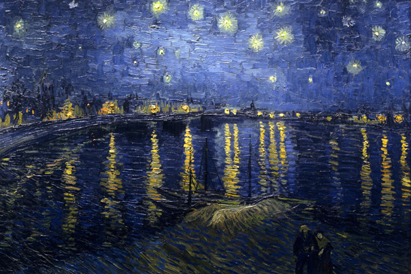
van Gogh – Starry Night Over the Rhone (September 1888)
In essence, the net knows absolutely nothing; it is blissfully ignorant of the real world. The system is trained using (typically many thousands of) pre-classified test images. The first image through the system is tentatively classified. Given no pre-knowledge at all, in a binary system, that very first pass has only a 50:50 chance of classifying correctly.
In effect, the system guesses.
Its guess is compared against the true classification for the image. Through a process called “back propagation”, the weights in each neuron (relating to which colours indicate day or night) are updated to gradually correct for errors, whenever it misclassifies. It is only after many thousands of training images that a classifier starts to get good in at its job. Eventually, the system reaches a stage of diminished returns, where additional training doesn’t improve accuracy any further. This is called converging.
Note that apart from shoveling images at it, such a system trains with little or no human intervention, and no hints as to what colours to look for. That is its great strength: no expert required. Salient characteristics are gradually intuited, i.e., “emerge” through repeated training sessions. Although it is possible, in some situations, to examine the neural net and discover what it is looking for (the colours of day and night being a credible, albeit simplified, example), in most cases the subtleties are too nuanced to properly understand.
A recently-published paper by Google DeepMind illustrates this point well.
PlaNet: Geolocating Photos Via Their Pixels
In mid-February 2016, a paper was published on Arxiv: PlaNet – Photo Geolocation with Convolutional Neural Networks. The paper describes a system that attempts to geolocate images based strictly on their pixel content.
This use of a “pixel-only” strategy was in fact fairly unique: previous systems had been coded to recognize salient landmarks, determine which side of the road cars were driving on, examine road-marking colourings, and so on: effectively, hand-coded rule-based systems. For this reason, such systems tended to have highly irregular success rates. For example, such systems tend to do much better in city centres than rural settings, because the former tend to be richer in unique landmarks and cultural clues. If the photo is of the Eiffel Tower, where it was taken is a no-brainer; on the other hand, if it is of a sunny, sandy beach, it could be on any continent except Antarctica.
PlaNet takes a completely different approach. It divides the Earth up into a bunch of geographically defined, non-overlapping cells. Cell-size is very roughly inversely proportional to population density, as city centres tend to be disproportionately represented in large photo libraries. There are abundant photos of the Statue of Liberty; not so many of that corn field in Wisconsin. For this reason, huge swathes of the oceans and the poles are simply not covered at all by the system. Some cells are enormous; some cells are quite small. The end result was 26,000, predominantly land-based cells, covering the hot-spots where most photos are taken.
The system was trained and tested using 126 million geotagged photos randomly mined from the web. You read right: “126 million”. Of these, 91 million where used for training, and 34 million for testing (all three figures are approximate; hence they don’t tally up exactly). An interesting point to note is the images underwent very little filtering: only non-photos (diagrams, clip-art) and pornography were eliminated. So the source images included portraits, pets, indoor shots, product packaging, and so on.
This means the training and test images were particularly challenging: how would you decide where that picture of a cat on a mat was taken?
In order to train the system, weights were initialized randomly, then images fed in. The output layer was effectively 26,000 neurons, one for each of the geographic cells. When an image is classified, each output neuron receives a probability value, representing how likely it is that the photo was taken in the geographic cell it represents. So, on output, the vast majority of those neurons will contain a value of very nearly 0. The cell with the highest probability value wins. However, many images will have several cells with close-to-highest probability scores: a beach in California might look very similar to one on the Mediterranean coast of southern France. So both might receive a relatively high score, and be close in value to each other.
Complexity and Accuracy
Straightaway, one can see this is many, many orders of magnitude more complex than the model I explained above; you’d need a very large piece of paper to draw its schematic. Training itself took 2.5 months, using 200 CPU cores. And they weren’t given weekends and holidays off.
But let’s cut to the bottom line: the system is surprisingly accurate. It achieved about 4% street-level accuracy (that is to say, in 4% of cases they nailed the very street the image came from), 10% city-level, and close to 30% country-level accuracy.
Although that might not sound all that great, it is worth remembering that photos were chosen more or less randomly from the web; they didn’t comprise just a long series of Eiffel Towers and Statues of Liberty. Photos could come from anywhere on the globe. Many photos from comparatively obscure places like Namibia/Botswana, Hawaii and the Galapagos Islands were accurately classified.
And don’t forget, that’s including cats on mats.
PlaNet consistently beat both versions of Im2GPS, a competing system, at all levels of geographic granularity, and likewise beat 10 “well-travelled humans”, winning 28 of 50 rounds of 5-photo tests.
Accuracy Does Not Equal Understanding
But for all its success, PlaNet cannot be said to understand anything. Like the simple Day/Night model I described above, at no point does the system ever arrive at concepts of “building” or “wild animal”, “mountain” or “road sign”, let alone “Eiffel Tower” or “Galápagos tortoise”. There are no such concepts in its vocabulary, because it has no vocabulary.
The actual question of whether we understand it is problematic as well. It is not exactly a black box — the foregoing proves in fact we have a tolerable understanding — but there is a very conceptually fuzzy bit in the middle, which is exactly where the emergent behaviour occurs.
First, we don’t really know exactly which characteristics it is looking at. The system contains millions of neurons, all beavering away on their own little corner of the image, all evaluating their own abstract feature. Unlike a rule-based system, it is not possible to say where a specific decision is getting made, or what path is taken through some decision tree. Instead, millions of mini-probabilities percolate up through the system, and help to arrive at a classification.
That is not to say we can never understand it. No doubt more sophisticated diagnostics will help the Google team ferret out the kinds of characteristics that prove useful in pin-pointing a photo’s location. But due to the incredible size and complexity of the system, how these characteristics interact will always be somewhat mysterious.
And it is telling that, at the moment, the system cannot be tweaked, at least in the normal sense of the word. If it gets some classification badly wrong, there is no way to kind of “lift the hood and tinker”. And performing more training is not going to help either: as stated earlier, the criterion for terminating training was in fact when the system started to converge on a ceiling value of accuracy.
In fact the only way forward for such a system is to start again: change some of the structural characteristics of the net, alter the algorithms for error reduction and back propagation, re-initialize all the weights to random values, and start re-training from scratch. And there is no guarantee that, 126 million images and two and a half months later, the result will be a better system. It could be worse.
Effectively: we’re just rolling the dice again.
Returning to Feynman
Let’s return to Feynman. His colleague, Murray Gell-Mann is said to have described Feynman’s own general problem-solving algorithm as follows:
- Write down the problem.
- Think really hard.
- Write down the answer.
This is of course an exaggeration, suggesting Feynman could consciously home directly in on a given solution, like some kind of heat-seeking missile. In reality, Feynman’s creative process must have involved its own effective “rolling the dice again”. He was notorious for changing his mind, particularly when the evidence changed. But he was, perhaps, adept at “loading the dice” on each throw, so they rolled more towards the direction he needed to go. Although he didn’t yet have an answer to the problem, he understood it in some deep way. So despite pitfalls and local dead ends, his “thinking really hard” always brought him closer to writing down the answer.
Richard Feynman
The current state-of-the-art in Artificial Intelligence does not yet posses anything like the same directional compass. When we roll the dice again each time, it really is a crap shoot. We can build these things, but the role that chance plays in their development proves that, at some deep, Feynmanian level, we really don’t understand them.
Creating is not understanding in Artificial Intelligence.
©2016 Brad Varey